Mastering Ridge Regression: A Key to Taming Data Complexity

Introduction

Whether you’re taking your first steps into the vibrant world of data science or you’ve already clocked some mileage, regression is a concept you can’t afford to overlook. Far more than just lines drawn on graphs, regression forms the backbone of many predictive analyses and data-driven decisions. Among the various forms of regression, Ridge Regression stands out as a powerful tool to tackle certain common issues in linear regression models.

In this article, we’ll dive into Ridge Regression, explore how it compares and contrasts with other regression techniques, and of course, put theory into practice with Python. If you’ve heard terms like “L2 penalty” or “lambda hyperparameter” but weren’t entirely sure what they meant or how they really mattered to your data model, you’re in the right place.

Understanding Ridge Regression

Ridge Regression, also known as Tikhonov regularization, is a technique used to analyze data afflicted by multicollinearity, a phenomenon where independent variables in a linear regression model are highly correlated. When multicollinearity is present, the estimated regression coefficients can become unstable, and the analysis overly sensitive to small variations in the data. This is where Ridge Regression comes in.

Unlike ordinary linear regression, which seeks to minimize the sum of the squares of the residuals (the difference between the observed and predicted values by the model), Ridge Regression adds a penalty term to the calculation. This penalty term is proportional to the square of the model coefficients, also known as the L2 norm of the coefficients. Mathematically, this translates to minimizing the following cost function:

Where:

• J(θ) is the Ridge cost function to be minimized.
• MSE(θ) is the mean squared error.
• λ is the regularization hyperparameter.
• θi are the model coefficients, with i ranging from 1 to n, the number of independent variables.

L1 vs L2 Penalty

In the quest to build more robust models less prone to overfitting, data science employs two main regularization techniques: L1 and L2. The L1 penalty, known by the Lasso (Least Absolute Shrinkage and Selection Operator) technique, not only regularizes but can also force some coefficients to be exactly zero, which equates to variable selection. This can be particularly useful when we suspect that some independent variables may be irrelevant or redundant.

On the other hand, the L2 penalty, which we use in Ridge Regression, doesn’t zero out coefficients but gradually reduces them, bringing them closer to zero and thus diminishing their influence on the model. This is especially useful in situations where all variables contribute to the prediction, but we want to penalize those with a lesser effect.

The choice between Lasso and Ridge will depend on the specific problem you’re trying to solve. Lasso might be the better option when we have many variables and suspect some might not be important, while Ridge might be preferable when all variables are considered significant.

The Role of the Lambda Hyperparameter

The hyperparameter λ plays a crucial role in the regularization of Ridge Regression models. It controls the strength of the penalty applied to the model coefficients. When λ is zero, Ridge Regression becomes an ordinary linear regression. As λ increases, the penalty on the coefficients also increases, and the values of the coefficients decrease towards zero. This can reduce overfitting as the model becomes less complex.

However, if λ is too high, the model can become overly simple and fail to capture the complexity of the data adequately, leading to underfitting. Therefore, the choice of λ is a balancing act: it should be large enough to regularize the effect of the predictor variables, but not so large that the model loses its predictive accuracy.

Selecting the optimal value of λ is usually done through techniques like cross-validation, where different values of λ are tested, and the value that results in the best prediction performance is chosen.

Practical Application: Ridge Regression with scikit-learn

Now let’s move from theory to practice and apply Ridge Regression to a real dataset with the help of scikit-learn, one of the most popular machine learning libraries in Python. Imagine we have a dataset containing several independent variables (X) and we want to predict a continuous output value (y).

from sklearn.linear_model import Ridge
from sklearn.model_selection import train_test_split
from sklearn.metrics import mean_squared_error
from sklearn.datasets import make_regression
import matplotlib.pyplot as plt
import numpy as np

# Generate a synthetic regression dataset
X, y = make_regression(n_samples=100, n_features=100, noise=0.1, random_state=42)

# Split the data into training and testing sets
X_train, X_test, y_train, y_test = train_test_split(X, y, test_size=0.2, random_state=42)

# Instantiate the Ridge Regression model
ridge_reg = Ridge(alpha=1)  # alpha is the hyperparameter equivalent to lambda

# Train the model
ridge_reg.fit(X_train, y_train)

# Make predictions
y_pred = ridge_reg.predict(X_test)

# Evaluate the model using mean squared error
mse = mean_squared_error(y_test, y_pred)
print(f"Mean Squared Error: {mse:.2f}")

# Print the first 10 coefficients to avoid a very long output
print("\nFirst 10 coefficients of the Ridge model:")
for i in range(10):
    print(f"Coefficient {i}: {ridge_reg.coef_[i]:.2f}")

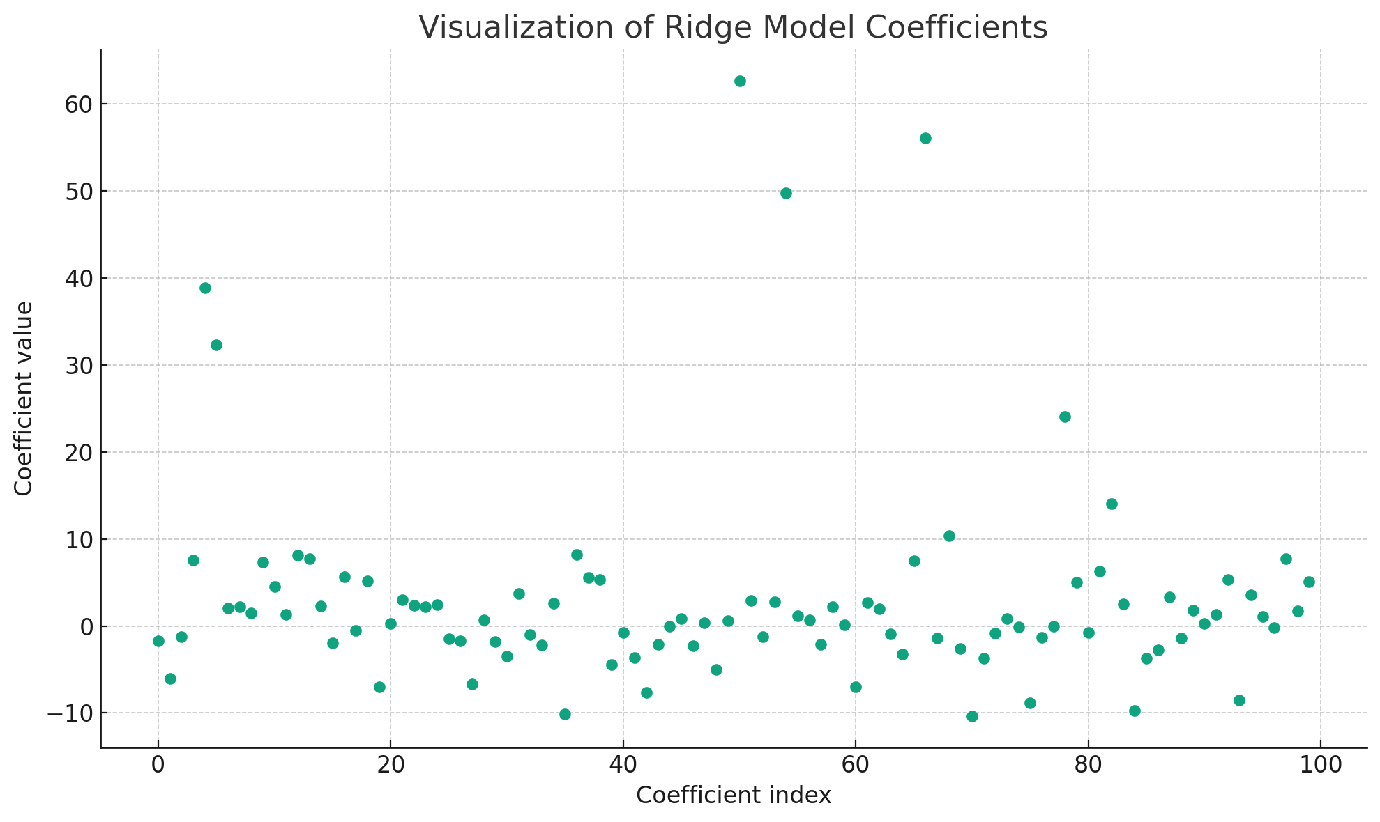
# Visualize the coefficients in a graph
plt.figure(figsize=(10, 6))
plt.plot(ridge_reg.coef_, marker='o', linestyle='')
plt.xlabel('Coefficient index')
plt.ylabel('Coefficient value')
plt.title('Visualization of Ridge Model Coefficients')
plt.tight_layout()  # Adjust the layout to avoid overlap
plt.grid(True)
plt.show()

In this example, we generated a synthetic dataset using the make_regression function from sklearn.datasets, which is commonly used for creating a regression problem with controllable noise and a number of features. After generating the data, we split it into training and test sets. We then instantiated the Ridge model from scikit-learn, where alpha is the parameter that controls the strength of regularization (equivalent to λ in theory). After training the model on the training data, we made predictions on the test data and evaluated the model using the mean squared error (MSE).

The Mean Squared Error (MSE) of the model on the test set is 4352.46.

Here are the first 10 coefficients of the Ridge model for illustrative purposes:

• Coefficient 0: -1.75
• Coefficient 1: -6.07
• Coefficient 2: -1.21
• Coefficient 3: 7.55
• Coefficient 4: 38.85
• Coefficient 5: 32.33
• Coefficient 6: 2.06
• Coefficient 7: 2.17
• Coefficient 8: 1.50
• Coefficient 9: 7.33

A graph was displayed to visualize the coefficients of the Ridge model. The plot reveals the influence of Ridge regularization, with some coefficients being pulled towards zero, reflecting their reduced impact on the model due to the L2 penalty. The graph helps in understanding which features have more weight and which are regularized more aggressively.

This practical example demonstrates how Ridge Regression can be applied to understand the relationship between features and an output variable in a dataset. The visualization of the coefficients serves as a valuable tool for interpreting the model and the effect of regularization.

Conclusion

Ridge Regression is a powerful and flexible modeling technique that can significantly improve the performance of linear regression models, particularly in situations where data exhibit multicollinearity. By balancing the need for model simplicity with adequate capture of data complexity, it allows us to create more generalizable and robust models.

With practice and a solid understanding of the concepts discussed here, you’ll be well-equipped to implement Ridge Regression in your own data science projects. Remember, the key to success with these models lies in experimentation and careful selection of hyperparameters.